The Hilbert curve can be used to serialize a two dimensional data
set. By walking along this curve all points are reached without
getting any of them twice. Although this transformation is a common
task in various applications it has to be reimplemented for every
individual data structure or application. The Dadim Api is suggested
standardization for the lacking concept of a mathematical function.
This section defines a Hilbert curve operator H which can be applied
to a 2D function and generates a data set containig all values of the
original function in one direction. The vertices of the Hilbert curve
can be generated by applying the operator H to the 2D identity
function.
Points
A vertex of the hilbert curve is encoded in a Point P. P evaluates to a
two dimensional vector and can be translated in the x and y direction.
Mathematically this is equivalent to the identity function in 2D space.
In the following examples P represents the data set to be serialized.
Rotation
The Rotation operator R rotates a Dadim f by 90 degrees.
Mirror
The Mirror operator M mirrors a Dadim f along the y direction.
Hilbert curve
The Hilbert curve operator H transforms a given Dadim f such that all
points of the hilbert curve are reached by traversing through Hf in
the h direction. Movements along x and y will be passed to function
which the curve operator H is applied to. If requiered, additional
dimensions x' and y', moving the original function f, could be
introduced. Thereby H transforms a 2D function into a 5D one. One
dimension h for the consecutive points on the hilbert curve. Two
dimensions moving the function in a coordinate system that is aligned
according to the current position in the hilbert curve and two
dimensions for the original carthesic standard coordinate system.
The Hilbert curve can be in 4 different stages, which will be denoted
by four different Hilbert curve operators H0 to H3.
Translating the Hilbert curve in the h direction produces the next point on
the curve.
Implementation
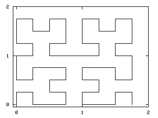
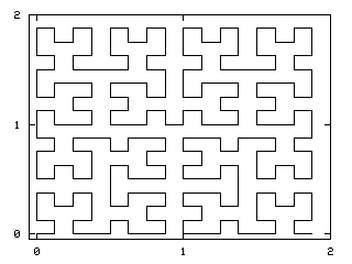
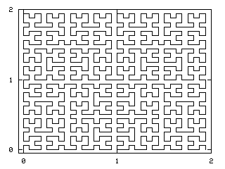
With the previously defined replacement rules we can easily compute a Hilbert curve of level
n:
Zh2n H0 P
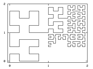
Adaptive Hilbert curves can be rendered by moving along the Hilbert curve and
apply the zoom operator whenever adaptive refinement is required. The zoom operator
is only defined if applied twice, since every refinement places four new points at the
position of one. Refinements are always combined in the x and y direction. Future
implementations of the operator might resolve these restrictions.
The Dadim Api can be used to implement Hilbert curves
There is a simple mathematical notation within the Dadim calculus
The Hilbert curve transformation can be implemented independed from
the underlying data structure and from the intended application. It can be applied
to data and functions.
The H operator preserves spacial dependecies, accessible via the x and y direction